By Long Luo

This article is the solution 4 Approaches: Brute Force, Exponent, Binary Search and the Newton’s Iteration Method of Problem 69. Sqrt(x).

Here shows 4 approaches for finding the square root of a number: Brute Force, Exponent, Binary Search and the Newton’s Iteration Method.

Given an integer \(N\) and a tolerance level \(L\), the task is to find the square root of that number.

Brute Force

The Brute Force way is very easy, just enumerate a value from \(0\) to \(x\), check the product \(i^2\) and target, return the answer.

1
2
3
4
5
6
7
8
9
10
11
12
13
14
15
16
17

public static int mySqrt(int x) {
    if (x == 0 || x == 1) {
        return x;
    }

    for (int i = 0; i < x; i++) {
        long sum = i * i;
        long bigger = (long) (i + 1) * (i + 1);
        if (sum == x) {
            return i;
        } else if (sum < x && bigger > x) {
            return i;
        }
    }

    return 0;
}

Analysis

• Time Complexity: \(O(n)\)
• Space Complexity: \(O(1)\).

Exponent

Noted that:

\[ \sqrt{x} = x^{1/2} = (e ^ {\ln x})^{1/2} = e^{\frac{1}{2} \ln x} \]

So we can use the exponent \(\exp\) and logarithm \(\ln\) to calculate the square root of the number \(\sqrt{x}\).

It’s really a fast and simple way!

Note: Since the computer can’t store the exact value of the float number, and the parameters and return values of the exponential function and logarithmic function are float numbers, so the result may be wrong.

For example, when \(x = 2147395600\), the result of \(e^{\frac{1}{2} \ln x}\) is \(10^{-11}\) from the correct value of \(46340\), so when taking the integer part of the result, you will get the wrong result of \(46339\).

So after getting the integer part \(\textit{ans}\) of the result, we should find out which of \(\textit{ans}\) and \(\textit{ans} + 1\) is the real answer.

1
2
3
4
5
6
7
8

// Exp O(1) O(1)
public static int mySqrt_exp(int x) {
    if (x == 0) {
        return 0;
    }
    int ans = (int) Math.exp(0.5 * Math.log(x));
    return (long) (ans + 1) * (ans + 1) <= x ? ans + 1 : ans;
}

Analysis

• Time Complexity: \(O(1)\)
• Space Complexity: \(O(1)\).

By Long Luo

This article is the solution Fast Power Algorithm: Binary Exponentiation of Problem 50. Pow(x, n).

We know how to find \(2.0\) raised to the power \(10\). The easiest way is to multiply \(10\) times \(2.0\) by loop, but what if we have to find \(2.0\) raised to the power very large number such as \(10000\) or more?

We will discuss how to find the solution of such problems by using an fast, efficient algorithm.

Brute Force

We multiply \(a\) to itself \(b\) times. That is, \(a^b = \underbrace{a \times a \dots \times a}_b\).

A simple java implementation of that would be:

1
2
3
4
5
6
7
8
9
10
11
12
13
14
15
16
17
18
19
20
21
22
23
24
25

public static double myPow(double x, int n) {
    if (n == 0 || x == 1) {
        return 1;
    } else if (x == 0) {
        return 0;
    }

    double ans = x;
    boolean isNegative = false;
    long nLong = n;
    if (nLong < 0) {
        nLong = -nLong;
        isNegative = true;
    }

    for (int i = 1; i < nLong; i++) {
        ans = ans * x;
    }

    if (isNegative) {
        ans = 1 / ans;
    }

    return ans;
}

Analysis

• Time Complexity: \(O(n)\)
• Space Complexity: \(O(1)\)

By Long Luo

傅里叶变换(Fourier Transform)是什么？

傅里叶变换 ¹ \((\textit{Fourier Transform})\) ² 和傅里叶级数 \((\textit{Fourier Series})\) ³ 是有史以来最伟大的数学发现之一。

傅里叶变换 \((\textit{Fourier Transform})\) 到底是什么，可以看下这个视频 形象展示傅里叶变换 ，讲的非常好。

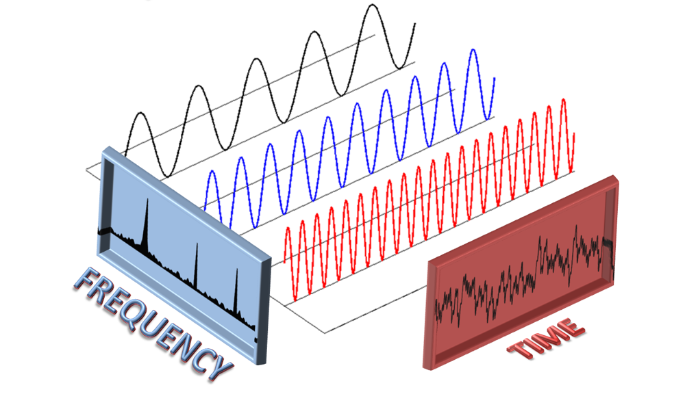
傅里叶级数和傅里叶变换背后的本质: 任何函数都可以写成正弦函数之和。

如下Gif动图所示：

下面这个视频 12分钟的傅立叶级数动画 ，我们可以看到任何图像都可以用大圆套小圆来绘制。

因为我们日常看到的世间万物都会随时间流逝而变化，比如一段声音，一幅图像或者一盏闪烁的交通灯，这种以时间作为参照来观察动态世界的方法我们称其为时域分析。

傅里叶告诉我们任何一个信号都可以用 \(2\) 种方式来表达：

1. 时域表达：自变量是时间或者空间的坐标，因变量是信号在该处的强度；
2. 频域表达：把信号“展开”成不同频率的简单正弦函数的叠加，相当于看作是定义在所有频率所组成的空间（称为频域空间）上的函数，自变量是不同的频率，因变量是该频率所对应的简谐振动的幅度。

这两个函数一个定义在时域（或空域）上，一个定义在频域上。看起来的样子通常截然不同，但是它们是在以完全不同的方式殊途同归地描述着同一个信号。它们就象是两种不同的语言，乍一听完全不相干，但是其实可以精确地互相翻译。在数学上，这种翻译的过程被称为傅立叶变换\((\textit{Fourier Transform})\) 。

傅里叶变换(Fourier Transform)可以做什么？

在傅立叶变换的所有这些数学性质中，最不寻常的是这样一种特性：一个在时域或空域上看起来很复杂的信号（譬如一段声音或者一幅图像）通常在频域上的表达会很简单。这里「简单」的意思是说作为频域上的函数，它只集中在很小一块区域内，而很大一部分数值都接近于零。例如下图是一张人脸和它对应的傅立叶变换，可以看出，所有的频域信号差不多都分布在中心周围，而大部分周边区域都是黑色的（即零）。

这是一个意味深长的事实，它说明一个在空域中看起来占满全空间的信号，从频域中看起来很可能只不过占用了极小一块区域，而大部分频率是被浪费了的。这就导出了一个极为有用的结论：一个看起来信息量很大的信号，其实可以只用少得多的数据来加以描述。只要对它先做傅立叶变换，然后只记录那些不接近零的频域信息就可以了，这样数据量就可以大大减少。

基本上，这正是今天大多数数据压缩方法的基础思想。在互联网时代，大量的多媒体信息需要在尽量节省带宽和时间的前提下被传输，所以数据压缩从来都是最核心的问题之一。而今天几乎所有流行的数据压缩格式，无论是声音的mp3格式还是图像的jpg格式，都是利用傅立叶变换才得以发明的。从这个意义上说来，几乎全部现代信息社会都建立在傅立叶的理论的基础之上。

关于不确定性原理，可以看下这个讲解的视频：直观看待不确定性原理：不只是量子现象哦 。

By Long Luo

卷积(Convolution)是什么？

卷积 ¹ \((\textit{Convolution})\) ² 是数学分析中一种重要的运算。

设：\(f(x)\) 、\(g(x)\) 是 \(\mathbb{R}\) 上的两个可积函数，作积分：

\[ \int _{-\infty }^{\infty }f(\tau)g(x-\tau)\,\mathrm{d}\tau \]

可以证明，关于几乎所有的 \(x \in (-\infty, \infty)\)，上述积分是存在的。这样，随着 \(x\) 的不同取值，这个积分就定义了一个新函数 \(h(x)\)，称为函数 \(f\) 与 \(g\) 的卷积，记为 \(h(x)=(f*g)(x)\)。

我们可以轻易验证： \((f \star g)(x)=(g \star f)(x)\)，并且 \((f \star g)(x)\) 仍为可积函数。这就是说，把卷积代替乘法，\(L^{1}(R^{1})\) 空间是一个代数，甚至是巴拿赫代数。

虽然这里为了方便我们假设 \(f, g\in L^{1}(\mathbb{R} )\)，不过卷积只是运算符号，理论上并不需要对函数 \(f,g\) 有特别的限制，虽然常常要求 \(f, g\) 至少是可测函数(measurable function) (如果不是可测函数的话，积分可能根本没有意义)，至于生成的卷积函数性质会在运算之后讨论。

卷积与傅里叶变换有着密切的关系。例如两函数的傅里叶变换的乘积等于它们卷积后的傅里叶变换，利用此一性质，能简化傅里叶分析中的许多问题。

由卷积得到的函数 \(f \star g\) 一般要比 \(f\) 和 \(g\) 都光滑。特别当 \(g\) 为具有紧支集的光滑函数，\(f\) 为局部可积时，它们的卷积 \(f \star g\) 也是光滑函数。利用这一性质，对于任意的可积函数 \(f\)，都可以简单地构造出一列逼近于 \(f\) 的光滑函数列 \(f_{s}\)，这种方法称为函数的光滑化或正则化。

卷积的概念还可以推广到数列、测度以及广义函数上去。

性质

各种卷积算子都满足下列性质：

交换律 \(f \star g = g \star f\)

结合律 \(f \star (g \star h)=(f \star g) \star h\)

分配律 \(f \star (g+h)=(f \star g)+(f \star h)\)

数乘结合律 \(a(f \star g)=(af) \star g=f \star (ag)\)

其中 \(a\) 为任意实数（或复数）。

微分定理 \((f \star g)={\mathcal{D}}f \star g=f \star {\mathcal{D}}g\)，

其中 \(Df\) 表示 \(f\) 的微分，如果在离散域中则是指差分算子，包括前向差分与后向差分两种：

前向差分：\({\mathcal{D}}^{+}f(n)=f(n+1)-f(n)\)

后向差分：\({\mathcal{D}}^{-}f(n)=f(n)-f(n-1)\)

卷积定理

函数卷积的傅里叶变换是函数傅里叶变换的乘积。即，一个域中的卷积相当于另一个域中的乘积，例如时域中的卷积就对应于频域中的乘积。

\(\textit{F}(f \star g) = \textit{F}(f) \cdot {\textit{F}}(g)\)

其中 \(\textit{F}(f)\) 表示 \(f\) 的傅里叶变换。

卷积定理 ³ 指出，函数卷积的傅里叶变换是函数傅里叶变换的乘积。即一个域中的卷积对应于另一个域中的乘积，例如时域中的卷积对应于频域中的乘积 ⁴。

\[ \mathcal{F}\{f \star g\} = \mathcal{F}\{f\} \cdot \mathcal{F}\{g\} \]

其中 \({\mathcal{F}}(f)\) 表示 \(f\) 的傅里叶变换。下面这种形式也成立：

\[ \mathcal{F}\{f \cdot g\}= \mathcal{F}\{f\} \star \mathcal{F}\{g\} \]

借由傅里叶逆变换 \(\mathcal{F}^{-1}\)，也可以写成

\[ f \star g= \mathcal{F}^{-1}\big\{\mathcal{F}\{f\}\cdot\mathcal{F}\{g\}\big\} \]

注意以上的写法只对特定形式定义的变换正确，变换可能由其它方式正规化，使得上面的关系式中出现其它的常数因子。

这一定理对拉普拉斯变换、双边拉普拉斯变换、Z变换、梅林变换和Hartley变换（参见Mellin inversion theorem）等各种傅里叶变换的变体同样成立。在调和分析中还可以推广到在局部紧致的阿贝尔群上定义的傅里叶变换。

利用卷积定理⁵可以简化卷积的运算量。对于长度为 \(n\) 的序列，按照卷积的定义进行计算，需要做 \(2n-1\) 组对位乘法，其计算复杂度为 \(O(n^{2})\) ；而利用傅里叶变换将序列变换到频域上后，只需要一组对位乘法，利用傅里叶变换的快速算法之后，总的计算复杂度为 \(O(nlogn)\)。这一结果可以在快速乘法计算中得到应用。

By Long Luo

Leetcode 1705. 吃苹果的最大数目 题目如下：

1
2
3
4
5
6
7
8
9
10
11
12
13
14
15
16
17
18
19
20
21
22
23
24
25
26
27
28
29
30

1705. 吃苹果的最大数目

有一棵特殊的苹果树，一连$n$天，每天都可以长出若干个苹果。在第$i$天，树上会长出apples[i]个苹果，这些苹果将会在days[i]天后（也就是说，第i + days[i]天时）腐烂，变得无法食用。也可能有那么几天，树上不会长出新的苹果，此时用apples[i] == 0且days[i] == 0表示。
你打算每天**最多**吃一个苹果来保证营养均衡。注意，你可以在这$n$天之后继续吃苹果。
给你两个长度为$n$的整数数组days和apples，返回你可以吃掉的苹果的最大数目。

示例 1：
输入：apples = [1,2,3,5,2], days = [3,2,1,4,2]
输出：7
解释：你可以吃掉7个苹果：
- 第一天，你吃掉第一天长出来的苹果。
- 第二天，你吃掉一个第二天长出来的苹果。
- 第三天，你吃掉一个第二天长出来的苹果。过了这一天，第三天长出来的苹果就已经腐烂了。
- 第四天到第七天，你吃的都是第四天长出来的苹果。

示例 2：
输入：apples = [3,0,0,0,0,2], days = [3,0,0,0,0,2]
输出：5
解释：你可以吃掉5个苹果：
- 第一天到第三天，你吃的都是第一天长出来的苹果。
- 第四天和第五天不吃苹果。
- 第六天和第七天，你吃的都是第六天长出来的苹果。
 

提示：
apples.length == n
days.length == n
1 <= n <= 2 * 10^4
0 <= apples[i], days[i] <= 2 * 10^4
只有在 apples[i] = 0 时，days[i] = 0 才成立

下面记录下我做这道题的思考过程：

暴力

很明显，每过一天，可能就有苹果过期，那么最好的方法是每天挑选最临近过期的苹果吃，这样才能吃到最多的苹果，于是新建一个二维数组，分别存储苹果个数和过期时间。

之后遍历这个数组，使用一个指针指向数组下标，一个 \(time\) 变量表示时间，时间每日递增，当苹果数 \(> 0\) 和未过期时苹果数 \(-1\)，如果不满足，数组下标\(idx++\)，代码如下所示：

1
2
3
4
5
6
7
8
9
10
11
12
13
14
15
16
17
18
19
20
21
22
23
24
25
26
27

public int eatenApples(int[] apples, int[] days) {
    int len = apples.length;
    int ans = 0;
    int[][] sorted = new int[len][2];
    for (int i = 0; i < len; i++) {
        sorted[i][0] = apples[i];
        sorted[i][1] = i + days[i];
    }

    Arrays.sort(sorted, (o1, o2) -> o1[1] - o2[1]);
    int time = 0;
    int idx = 0;
    while (idx < len) {
        while (idx < len && (sorted[idx][0] <= 0 || sorted[idx][1] <= time)) {
            idx++;
        }

        if (idx < len && sorted[idx][1] > time) {
            sorted[idx][0]--;
            ans++;
        }

        time++;
    }

    return ans;
}

但是，这个方法只通过了 \(50\) 个test cases，遇到下列用例就不适用了：

1
2

[2,1,1,4,5]
[10,10,6,4,2]

那么问题出在什么地方呢？

因为排序结果会导致我们先吃了还没有长出来的果实，所以此方法不可行，需要修改。