By Long Luo

The \(\textit{Fibonacci Sequence}\)¹ are the numbers in the following integer sequence:

\(1, 1, 2, 3, 5, 8, 13, 21, 34, 55, 89, 144, 233, \dots\)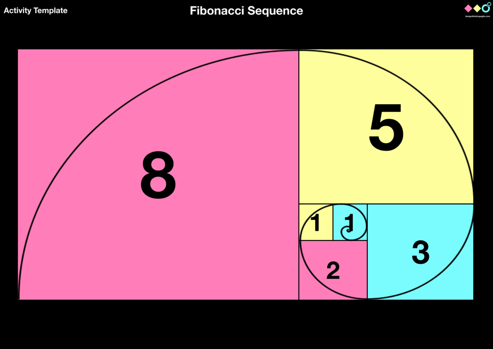

We can see the fibonacci series seqences in the natrual world like the sunflower, the nautilus and the galaxy.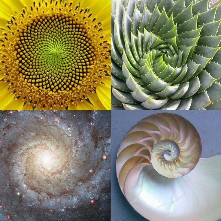

In mathematical terms, the sequence \(F(n)\) of Fibonacci numbers is defined by the recurrence relation

\[ F(n)=F(n-1)+F(n-2) \]

with seed values \(F(0) = 0\) and \(F(1) = 1\).

The Fibonacci sequence is often used in introductory computer science courses to explain recurrence relations, dynamic programming, and proofs by induction. Because the Fibonacci sequence is central to several core computer science concepts, the following programming problem has become fairly popular in software engineering interviews.

Given an input \(n\), return the \(nth\) number in the Fibonacci sequence.

Below I’ve listed \(9\) approaches to this problem. These different solutions illustrate different programming and algorithmic techniques that can be used to solve other problems. You’ll notice that many of these solutions build from previous solutions.

Solution 1 Lookup Table - 32 bit signed integers only

If we don’t need to solve very large values and are time-sensitive, we can calculate all values in advance.

This function will work strictly in the case that we’re dealing with \(32\) bit signed integers (which could be a constraint in languages like Java, C/C++, etc.)

The Fibonacci sequence grows very quickly. So fast, that only the first \(47\) Fibonacci numbers fit within the range of a \(32\) bit signed integer. This method requires only a quick list lookup to find the nth Fibonacci number, so it runs in constant time. Since the list is of fixed length, this method runs in constant space as well.

1
2
3
4
5
6
7
8
9
10
11
12

class Solution {
    int[] fib_nums = {
            0, 1, 1, 2, 3, 5, 8, 13, 21, 34, 55, 89, 144, 233, 377, 610, 987, 1597, 2584, 4181,
            6765, 10946, 17711, 28657, 46368, 75025, 121393, 196418, 317811, 514229, 832040,
            1346269, 2178309, 3524578, 5702887, 9227465, 14930352, 24157817, 39088169, 63245986,
            102334155, 165580141, 267914296, 433494437, 701408733, 1134903170, 1836311903
    };

    public int fib(int n) {
        return fib_nums[n];
    }
};

Analysis

• Time Complexity: \(O(1)\)
• Space Complexity: \(O(1)\)

Solution 2 Recursion

A simple method that is a direct recursive implementation mathematical recurrence relation is given above.

1
2
3
4
5
6
7
8

//Fibonacci Series using Recursion
public static int fib(int n) {
	if (n <= 1) {
		return n;
	}

	return fib(n - 1) + fib(n - 2);
}

Analysis

• Time Complexity: \(O(\phi^n)\), where \(\phi\) is the golden ratio (\(\phi \simeq 1.618...\)).

If we count the number of calls that this algorithm makes for any n, we will find its runtime complexity.

Let \(T(n)\) refer to the number of calls to fib1 that are required to evaluate fib1(n).

When fib1(0) or fib1(1) is called, fib1 doesn’t make any additional recursive calls, so \(T(0)\) and \(T(1)\) must equal 1.

For any other n, when fib1(n) is called, fib1(n - 1) and fib1(n - 2) are also called.

So

\[ T(n) = 1 + T(n - 1) + T(n - 2) \]

Using more advanced mathematical techniques, like generating functions, one can solve the recurrence \(T\), and find that \(T\) scales as \(O(\phi)\).

If the original recursion tree were to be implemented then this would have been the tree but now for n times the recursion function is called.

Original tree for recursion:

1
2
3
4
5
6
7
8
9

                          fib(5)   
                     /                \
               fib(4)                fib(3)   
             /        \              /       \ 
         fib(3)      fib(2)         fib(2)   fib(1)
        /    \       /    \        /      \
  fib(2)   fib(1)  fib(1) fib(0) fib(1) fib(0)
  /     \
fib(1) fib(0)

Optimized tree for recursion for code above:

1
2
3
4
5

fib(5) 
fib(4)
fib(3)
fib(2)
fib(1)

• Space Complexity: \(O(n)\) if we consider the function call stack size, otherwise \(O(1)\).

Solution 3 Dynamic Programming

We can avoid the repeated work done in Recursion solution by storing the Fibonacci numbers calculated so far.

1
2
3
4
5
6
7
8
9
10
11
12
13
14
15
16
17

// Dynamic Programming
public int fib(int n) {
	/* Declare an array to store Fibonacci numbers. */
	int f[] = new int[n + 1]; // 1 extra to handle case, n = 0
	int i;

	/* 0th and 1st number of the series are 0 and 1*/
	f[0] = 1;
	f[1] = 1;

	for (i = 2; i <= n; i++) {
		/* Add the previous 2 numbers in the series and store it */
		f[i] = f[i - 1] + f[i - 2];
	}

	return f[n];
}

Analysis

• Time Complexity: \(O(n)\)
• Space Complexity: \(O(n)\)

Solution 4 DP using memoization(Top down approach)

We can avoid the repeated work done in Solution 2 Recursion by storing the Fibonacci numbers calculated so far. We just need to store all the values in an array.

1
2
3
4
5
6
7
8
9
10
11
12
13
14
15
16
17
18
19
20
21
22
23
24
25
26

// Initialize array of dp
public static int[] dp = new int[31];

public static int fib(int n) {
    if (n <= 1) {
        return n;
    }

    // Temporary variables to store values of fib(n-1) & fib(n-2)
    int first, second;

    if (dp[n - 1] != -1) {
        first = dp[n - 1];
    } else {
        first = fib(n - 1);
    }

    if (dp[n - 2] != -1) {
        second = dp[n - 2];
    } else {
        second = fib(n - 2);
    }

    // Memoization
    return dp[n] = first + second;
}

Analysis

• Time Complexity: \(O(n)\)
• Space Complexity: \(O(n)\)

Solution 5 Iterative (Space Optimized Method 3)

We can optimize the space used in Solution 3 Dynamic Programming by storing the previous two numbers only because that is all we need to get the next Fibonacci number in series.

This solution is one of the simplest and most efficient algorithms on this list. This function has a loop that runs through n iterations before returning, and each iteration does constant work, making the algorithm run in \(O(n)\) time. This function doesn’t use any extra data structures, and it isn’t recursive, so we can say that it uses \(O(1)\) space.

1
2
3
4
5
6
7
8
9
10
11
12
13
14
15

// Fibonacci Series using Space Optimized Method
class Solution {
    public int fib(int n) {
        if (n < 2) {
            return n;
        }
        int p = 0, q = 0, r = 1;
        for (int i = 2; i <= n; ++i) {
            p = q; 
            q = r; 
            r = p + q;
        }
        return r;
    }
}

Analysis

• Time Complexity: \(O(n)\)
• Space Complexity: \(O(1)\)

Solution 6 Recurrence Matrix

This is the most mathematical solution, and it requires some basic understanding of matrix multiplication.

Consider the following matrix \(M\):

\[ M = \begin{bmatrix} 1 & 1 \\ 1 & 0 \\ \end{bmatrix} \]

If \(f_{i-1}\) and \(f_{i-2}\) are the \(i-1\)th and the \(i-2\)th Fibonacci numbers, the following matrix product can give us the ith Fibonacci number \(f_{i}\):

\[ M * \begin{bmatrix} f_{i - 2} \\ f_{i - 1} \end{bmatrix} = \begin{bmatrix} f_{i - 1} \\ f_{i - 1} + f_{i - 2} \end{bmatrix} = \begin{bmatrix} f_{i - 1} \\ f_{i} \end{bmatrix} \]

Using this property of \(M\), one can find \(f_{n}\) by computing the product

\[ M^n \cdot \begin{bmatrix} f_0 \\ f_1 \end{bmatrix} = M^n \cdot \begin{bmatrix} 0 \\ 1 \end{bmatrix} \]

and returning the first element of the vector.

1
2
3
4
5
6
7
8
9
10
11
12
13
14
15
16
17
18
19
20
21
22
23
24
25
26
27
28
29
30
31
32
33
34
35
36
37
38

class Solution {
    public static int fib(int n) {
        int F[][] = new int[][]{{1, 1}, {1, 0}};
        if (n == 0) {
            return 0;
        }
        power(F, n - 1);
        return F[0][0];
    }

    /* Helper function that multiplies 2 matrices F and M of size 2*2, and
    puts the multiplication result back to F[][] */
    public static void multiply(int F[][], int M[][]) {
        int x = F[0][0] * M[0][0] + F[0][1] * M[1][0];
        int y = F[0][0] * M[0][1] + F[0][1] * M[1][1];
        int z = F[1][0] * M[0][0] + F[1][1] * M[1][0];
        int w = F[1][0] * M[0][1] + F[1][1] * M[1][1];

        F[0][0] = x;
        F[0][1] = y;
        F[1][0] = z;
        F[1][1] = w;
    }

    /* Helper function that calculates F[][] raise to the power n and puts the
    result in F[][]
    Note that this function is designed only for fib() and won't work as general
    power function */
    public static void power(int F[][], int n) {
        int i;
        int M[][] = new int[][]{{1, 1}, {1, 0}};

        // n - 1 times multiply the matrix to {{1,0},{0,1}}
        for (i = 2; i <= n; i++) {
            multiply(F, M);
        }
    }
}

Analysis

• Time Complexity: \(O(n)\)
• Space Complexity: \(O(1)\)

Solution 7 Fast Matrix Power(Optimized Method 6)

The Solution 6 Recurrence Matrix can be optimized to work in \(O(logn)\) time complexity. We can do recursive multiplication to get \(\texttt{power}(M, n)\) in the previous method (Similar to the optimization done in this post).

The key here is to compute \(M^n\) using the successive square method. Using this algorithm, \(M^n\) is computed in \(O(logn)\) time(Note that for a fixed matrix size, the matrix muliplication algorithm takes a constant amount of time).

Then, \(M^n\) is multiplied by \(\begin{bmatrix} 0 \\ 1 \end{bmatrix}\), and the top elemen of the product is returned.

This algorithm uses \(O(logn)\) to compute \(M^n\), and constant space, as the intermediary matricies can be reclaimed by the garbage collecter.

1
2
3
4
5
6
7
8
9
10
11
12
13
14
15
16
17
18
19
20
21
22
23
24
25
26
27
28
29
30
31
32

class Solution {
    public int fib(int n) {
        if (n < 2) {
            return n;
        }
        int[][] q = {{1, 1}, {1, 0}};
        int[][] res = pow(q, n - 1);
        return res[0][0];
    }

    public int[][] pow(int[][] a, int n) {
        int[][] ret = {{1, 0}, {0, 1}};
        while (n > 0) {
            if ((n & 1) == 1) {
                ret = multiply(ret, a);
            }
            n >>= 1;
            a = multiply(a, a);
        }
        return ret;
    }

    public int[][] multiply(int[][] a, int[][] b) {
        int[][] c = new int[2][2];
        for (int i = 0; i < 2; i++) {
            for (int j = 0; j < 2; j++) {
                c[i][j] = a[i][0] * b[0][j] + a[i][1] * b[1][j];
            }
        }
        return c;
    }
}

Analysis

• Time Complexity: \(O(logn)\).
• Space Complexity: \(O(logn)\), if we consider the function call stack size, otherwise \(O(1)\).

Solution 8 O(logn) Time

Below is one more interesting recurrence formula that can be used to find nth Fibonacci number in \(O(logn)\) time.

If \(n\) is even then \(k = n/2\):

\[ F(n) = [2F(k-1) + F(k)] \cdot F(k) \]

If \(n\) is odd then \(k = (n + 1)/2\)

\[ F(n) = F(k)F(k) + F(k-1)F(k-1) \]

How does this formula work?

The formula can be derived from above matrix equation.

\[ A^n=\begin{pmatrix} F_{n+1},&F_n \\ F_n,&F_{n-1} \end{pmatrix} \]

Taking determinant on both sides, we get:

\[ (-1)^n = F_{n+1}F_{n-1} - F_n^2 \]

Moreover, since \(A^nA^m = A^{n+m}\) for any square matrix \(A\), the following identities can be derived (they are obtained form two different coefficients of the matrix product)

\[ F_mF_n + F_{m-1}F_{n-1} = F_{m+n-1} ------(8.1) \]

By putting \(n=n+1\) in equation (8.1),

\[ F_mF_{n+1} + F_{m-1}F_n = F_{m+n} ------(8.2) \]

Putting \(m = n\) in equation(8.1).

\[ F_{2n-1} = F_n^2 + F_{n-1}^2 \]

Putting \(m = n\) in equation(8.2)

By putting: \(F_{n+1} = F_n + F_{n-1}\)

\[ F_{2n} = (F_{n-1} + F_{n+1})Fn = (2F_{n-1} + F_n)F_n \]

To get the formula to be proved, we simply need to do the following

If \(n\) is even, we can put \(k = n/2\) If \(n\) is odd, we can put \(k = (n+1)/2\)

Below is the implementation of above idea.

1
2
3
4
5
6
7
8
9
10
11
12
13
14
15
16
17
18
19
20
21
22
23
24
25
26

public static int MAX = 1000;
public static int f[];

// Returns n'th fibonacci number using
// table f[]
public static int fib(int n) {
    if (n == 0) {
        return 0;
    }

    if (n == 1 || n == 2) {
        return (f[n] = 1);
    }

    // If fib(n) is already computed
    if (f[n] != 0) {
        return f[n];
    }

    int k = (n & 1) == 1 ? (n + 1) / 2 : n / 2;

    // Applying above formula [Note value n&1 is 1 if n is odd, else 0.
    f[n] = (n & 1) == 1 ? (fib(k) * fib(k) + fib(k - 1) * fib(k - 1)) : (2 * fib(k - 1) + fib(k)) * fib(k);

    return f[n];
}

Analysis

• Time Complexity: \(O(logn)\) as we divide the problem to half in every recursive call.
• Space Complexity: \(O(logn)\)

Solution 9 Math Formula

We first look at the equation:

\[ F(n)=F(n-1)+F(n-2) ------(9.1) \]

To solve (9.1) for the Fibonacci numbers, we first look at the equation

\[ x_{n+1} = x_n + x_{n-1} ------(9.2) \]

This equation is called a second-order, linear, homogeneous difference equation with constant coefficients, and its method of solution closely follows that of the analogous differential equation.

Our idea is to guess the general form of a solution, find two such solutions, and then multiply these solutions by unknown constants and add them. This results in a general solution to (9.2), and one can then solve by satisfying the specified initial values.

To begin, we guess the form of the solution as

\[ x_n = λ^n ------(9.3) \]

where \(λ\) is an unknown constant.

Substitution of this guess into the equation, results in:

\[ λ^{n+1} = λ^n + λ^{n-1} \]

or upon division by \(λ^{n-1}\) and rearrangement of terms,

\[ λ^2 - λ - 1 = 0 \]

Use of the quadratic formula yields two roots, both of which are already familiar. We have:

\[ λ_1 = \frac{1+\sqrt{5}}{2} \]

\[ λ_2 = \frac{1-\sqrt{5}}{2} \]

We have thus found two independent solutions to (9.2) of the form (9.3), and we can now use these two solutions to find a solution to (9.1). Multiplying the solutions by constants and adding them, we obatin:

\[ F(n)=c_1λ_1^n + c_2λ_2^n \]

which must satisfy the initial values \(F(0)=1\)，\(F(1)=1\).

Application of the values for \(F0\) and \(F1\) results in the system of equations given by

\[ c_1 + c_2 = 0 \]

\[ c_1λ_1 - c_2λ_2 = 1 \]

we can solve for \(c_1\) and \(c_2\) to obtain:

\(c_1 = \frac{1}{\sqrt{5}}\)，\(c_2 = -\frac{1}{\sqrt{5}}\).

then derives the surprising formula:

\[ F(n)=\frac{1}{\sqrt{5}}\left[ \left(\frac{1+\sqrt{5}}{2}\right)^{n} - \left(\frac{1-\sqrt{5}}{2}\right)^{n} \right] \]

known as Binet’s formula.

In this method we directly implement the formula for nth term in the fibonacci series.

1
2
3
4
5
6
7

class Solution {
    public int fib(int n) {
        double sqrt5 = Math.sqrt(5);
        double fibN = Math.pow((1 + sqrt5) / 2, n) - Math.pow((1 - sqrt5) / 2, n);
        return (int) Math.round(fibN / sqrt5);
    }
}

Analysis

• Time Complexity: \(O(logn)\), this is because calculating \(phi^n\) takes \(logn\) time
• Space Complexity: \(O(1)\).

References

All suggestions are welcome. If you have any query or suggestion please comment below. Please upvote👍 if you like💗 it. Thank you:-)

Explore More Leetcode Solutions. 😉😃💗